Models for image processing and the visual domain in general are the flagships riding the deep learning wave today. Models for the auditive domain have not yet shown quite the same level of effectiveness, mostly due to the enormous range of timescales constituting meaningful sound (from fractions of milliseconds to minutes or even longer). Nevertheless there have been breakthroughs, most notably the WaveNet architecture, developed by Google DeepMind in 2016. WaveNet uses a computational module called dilated convolution to capture longer sequences. The size of the receptive field, i.e. the snippet of sound the network can access, increases exponentially with the number of layers. A typical WaveNet has a receptive field of several thousand samples, or a few hundred milliseconds . Of course this is not enough to include the many long-term dependencies that are so crucial in music. But it is sufficient for generating single words or syllables of speech. And indeed WaveNet has proven itself to be very successful for speech synthesis, being now used on a global scale for the voice of the Google assistant.
In this project I consider a way to adapt WaveNet for a more musical use. We can draw inspiration from from the psychology of human music perception. As it turns out, the processing of sound in the brain can be split into at least two types. The first type captures short time spans of a length in the hundreds of milliseconds. This corresponds to the WaveNet. But there is another type that holds longer sequences, i.e. several, up to 20 or more seconds (Cowan, 1987). Alternatively the term “perceptual present” is used for this second type, which lies right at the boundary between perception and reconstruction from memory. The majority of the evidence suggests that the perceptual presence lasts about 3-8 seconds (Clarke, 1999). Of course artificial neural networks have no actual sense of temporal presence (at least not yet). Here I suggest a mechanism that approximates something of similar effect in a straightforward way.
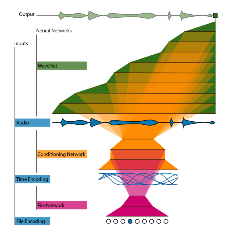
Usually, WaveNet is trained with thousands of short sections from a collection of audio files. No information is given concerning which file or where in the file this section comes from. The aim of this project is allowing the model to use exactly this information. The position of the audio section in the file is represented by a time encoding. This encoding has to uniquely represent each position in time, has to be continuous, and cannot give preference to any specific position. A collection of harmonic cosine and sine waves fulfills these requirements. It is well known that harmonic cosines and sines can be linearly transformed to represent any continuous function up to a certain level of detail. The lowest frequency is given by the length of the longest file, the highest frequency by the level of detail we want to represent, in our case determined by the perceptual present (in the following experiment I chose 8 seconds). This time encoding is fed into the conditioning network which warps the input into a form that accounts for the structure of the audio file. This structure information is then projected to each layer of the WaveNet, allowing it to generate sound that fits into the larger scale of the music. This process is called conditioning. In the speech synthesis setting, readily available phonetic information of the words to be synthesized is typically used as conditioning. Here we learn the conditioning directly from the data using the conditioning network.
If we only used the time encoding, the conditioning network would learn the same structure for each file in the training set. Of course this doesn’t make sense. So we need the file network, that gets as input the identity of the file as a one-hot-encoding and projects useful information for this file into the conditioning network. We now have a hierarchical architecture with three sub-networks, processing structures of increasing scale: The WaveNet handles fractions of a second, the conditioning network several seconds, and the file network minutes. The whole architecture is completely differentiable and can be trained en bloc.

This experiment uses as dataset the three movements of the piano sonata KV 331 in A-major by Wolfgang Amadeus Mozart. For implementation details, please see the github repository. The time encoding is illustrated in Figure 1. High frequencies are dampened to encourage the conditioning network to focus on long-term structure. The background colors represent the internal structure of each movement (first movement blue, second movement green, third movement red/yellow). It was manually added later, the network had no access to this information. We can visualize the output of the conditioning network by reducing it to two dimensions (using principal component analysis) and plotting the path the piece takes through this space. Points that are close to one-another should represent sections of the piece that are related in some way.

The first movement is a theme with six variations. We see that each variation has its own cluster, with the centers of the clusters gradually moving away from the theme.

The second movement has the structure **ABCDAB**. After part D, we move all the way to the left, where the second part A start. In the y direction both parts A and B are virtually indistinguishable, but they occupy different spaces in the x direction. This might suggest subtle differences between the original and the recapitulation of the parts, but it also may well be a training artifact.

The third movement is the famous “Rondo alla turca” (with the structure **ABCBAB*D**). Here the learned structure is clearly visible. All parts are well defined and the repeated parts are located at exactly the same positions. This suggests that the conditioning network recognizes the recurrence and actually “remembers” them. This is a first experiment, further experiments and audio samples will follow soon.
References
- Clarke, E. F. (1999). Rhythm and Timing in Music. In The Psychology of Music (2nd ed.), ed. Diana Deutsch, 473–500. San Diego: Academic Press.
- Cowan, N. (1987). Auditory memory: Procedures to examine two phases. In W. A. Yost & C. S. Watson (Eds.), Auditory processing of complex sounds (pp. 289-298). Hillsdale, NJ, US: Lawrence Erlbaum Associates, Inc.